(Thanks Jason Gross and Damon Binder for helping me with this. Epistemic status: I am not good at fiddly math; I am 90% confident that there are errors in the equations, but I am 75% confident that my qualitative arguments are right. I basically never bothered normalizing the wavefunctions. I found this reasoning useful for my own understanding, but I don’t know if it will be at all helpful for others.)
I’m interested in getting a deeper understanding of the time-dependent Schrödinger equation in one dimension:
$^$i\hbar \frac{d}{dt} \Psi(x) = \left(\frac{-\hbar^2}{2m}\nabla^2 + V(x)\right) \Psi(x)$^$
\(\Psi\) is of course a complex-valued function. We can write this equation instead as a pair of coupled real-valued functions for the real and imaginary parts of \(\Psi\):
$^$\hbar \frac{d}{dt} \operatorname{Re}(\Psi)(x) = -\left(\frac{-\hbar^2}{2m}\nabla^2 + V(x)\right) \operatorname{Im}(\Psi(x))$^$
$^$\hbar \frac{d}{dt} \operatorname{Im}(\Psi)(x) = \left(\frac{-\hbar^2}{2m}\nabla^2 + V(x)\right) \operatorname{Re}(\Psi(x))$^$
I think it’s helpful to try expressing the amplitudes in radial form (\(\Psi = r \cdot e^{i\theta}\)) rather than in this \(z = a + bi\) form. For this exercise, we’re only going to bother considering things in one dimension, so substitute \(\frac{d}{dx}\) for \(\nabla\).
I had a bit of trouble with the algebra, but Jason Gross helped me with it, and I then checked with Sympy, leaving me relatively confident in the following equations:
$^$\begin{align} \frac{d\theta}{dt} &= \frac{1}{m\hbar}\left(-mV + \frac{\hbar^2}{2} \left( - \left(\frac{d\theta}{dx}\right)^2 + \frac{1}{r}\frac{d^2r}{dx^2} \right)\right) \\ \frac{dr}{dt} &= \frac{-\hbar}{2m} \left(r\frac{d^2\theta}{dx^2} + 2 \frac{dr}{dx}\frac{d\theta}{dx}\right) \end{align} $^$
I think that this form makes several aspects of the behavior of the Schrödinger equation more intuitive.
Gaussian wavepackets
Let’s look at how the Schrödinger equation leads to a particle travelling along at a constant velocity in a region of constant potential.
Consider a wavefunction given by something like:
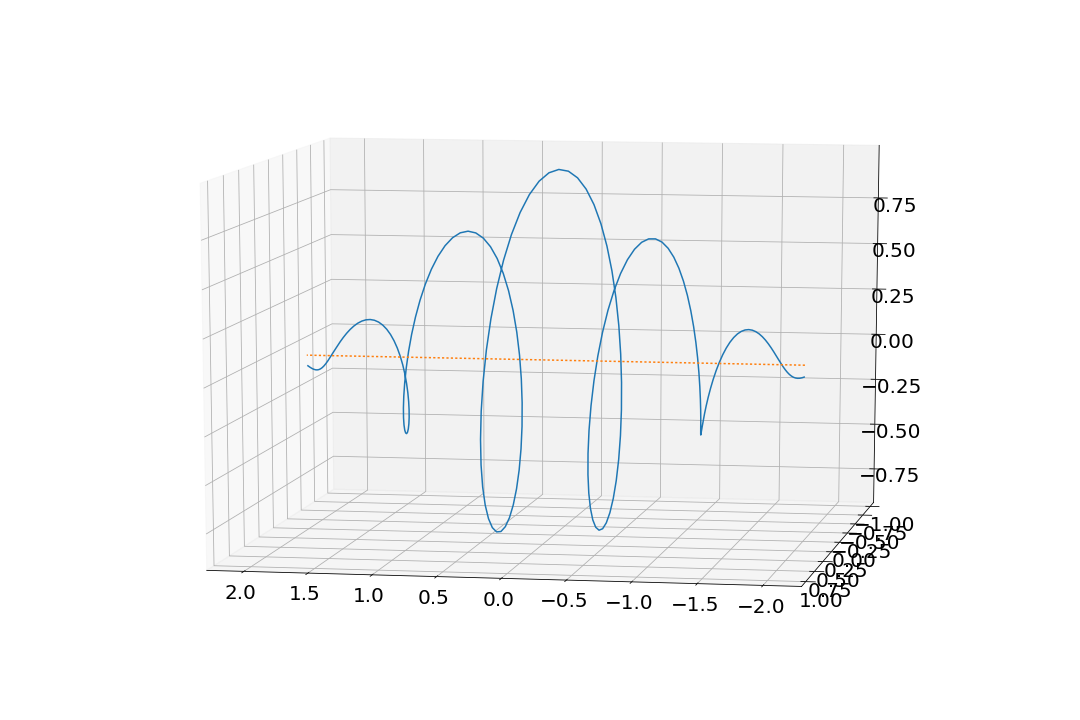
$^$\Psi(x) = e^{ipx} \cdot e^{-x^2}$^$
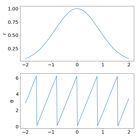
where \(p\) is a real number. If we write the amplitude down in radial coordinates, it becomes \(r(x) = e^{-x^2}, \theta(x) = px\).
It looks like this:
If we plot it in terms of \(r\) and \(\theta\), it looks like this:
Let’s look at the radial form of the Schrödinger equation again:
$^$\begin{align} \frac{d\theta}{dt} &= \frac{1}{m\hbar}\left(-mV + \frac{\hbar^2}{2} \left( - \left(\frac{d\theta}{dx}\right)^2 + \frac{1}{r}\frac{d^2r}{dx^2} \right)\right) \\ \frac{dr}{dt} &= \frac{-\hbar}{2m} \left(r\frac{d^2\theta}{dx^2} + 2 \frac{dr}{dx}\frac{d\theta}{dx}\right) \end{align} $^$
In this case, \(\theta\) is a linear function, so we can remove the \(\frac{d^2\theta}{dx^2}\). And we’re considering the case of a constant potential, so we might as well set \(V=0\). Removing those terms, we’re left with:
$^$\begin{align} \frac{d\theta}{dt} &= \frac{\hbar}{2m}\left( - \left(\frac{d\theta}{dx}\right)^2 + \frac{1}{r}\frac{d^2r}{dx^2} \right) \\ \frac{dr}{dt} &= \frac{-\hbar}{m} \frac{dr}{dx}\frac{d\theta}{dx} \end{align} $^$
Furthermore, let’s consider the case where \(p\) is large, so \(\theta\) is rapidly changing with \(x\). In this case, \(\frac{d\theta}{dx}\) is much greater than \(\frac{dr}{dx}\). So the RHS of the equation for \(\frac{d\theta}{dt}\) is roughly constant. This means that the wavefunction is rotating through the phase space at roughly the same rate across all of the wavefunction.
Now let’s look at the equation for \(\frac{dr}{dt}\). \(\frac{d\theta} {dx}\) is given by \(p\). If \(p\) is positive, the wavefunction is growing in all the regions where \(\frac{dr}{dx}\) is negative, and it is decreasing in all the regions where \(\frac{dr}{dx}\) is positive. Let’s quickly plot \(-\frac{dr}{dx}\):

So the wavepacket is increasing its amplitude to the right of its center, and decreasing it to the left. This suggests that the wavefunction is moving to the right.
How fast is it moving to the right? Let’s do this real sketchily. In the rest of this section, I’m going to ignore hbars and dimensional consistency. Let’s assume that our wavefunction is moving to the right at some speed \(v\), so that \(r(x, t)\) is given by:
$^$r(x,t) = \exp(-(x - t v)^2)$^$
We can differentiate this with respect to time, and we get:
$^$\frac{dr}{dt} = - 2 v \left(t v - x\right) e^{- \left(t v - x\right)^{2}}$^$
At \(t=0\), this reduces to \(2 v x e^{- x^{2}}\). We can equate this expression for \(\frac{dr}{dt}\) with the one we got above, which gives us
$^$-\frac{1}{m} \frac{dr}{dx}\frac{d\theta}{dx} = 2 v x e^{- x^{2}}$^$
In this case, \(\frac{dr}{dx} = - 2 x e^{- x^{2}}\), so we can cancel that out, leaving us with
$^$\frac{1}{m} \frac{d\theta}{dx} = v$^$
Remember that \(\frac{d\theta}{dx} = p\). This looks like \(p = m v\) to me, which is comforting.
Anyway, apparently this is why Gaussian wavepackets move along–they spiral around phase space while growing towards the regions where their spatial derivative of phase disagrees with their spatial derivative of amplitude.
Particles in potentials
Now let’s think about a particle in a linear potential, \(V = k x\). Imagine we have a Gaussian wavepacket without any particular momentum, with the wavefunction \(\Psi(x) = \exp(-x^2)\).
The potential only appears in the phase part of the radial form of the Schrödinger equation:
$^$\frac{d\theta}{dt} = \frac{1}{m\hbar}\left(-mV + \frac{\hbar^2}{2} \left( - \left(\frac{d\theta}{dx}\right)^2 + \frac{1}{r}\frac{d^2r}{dx^2} \right)\right) $^$
In the case where \(k\) is large, then the effect of the potential is just to twist the wavefunction around. Once it’s twisted around, it starts moving along for the reasons we discussed in the previous section.
In the case where \(k\) is positive, then the wavefunction will end up twisted such that \(\frac{d\theta}{dx}\) is negative, because the parts of the wavefunction further to the right end up rotated to a more negative \(\theta\). This leads to the wavefunction evolving towards the direction of lower potential.
I now feel like I understand what’s happening when you have a particle in a potential–it gets twisted around by the potential, and once it’s twisted, it propagates towards the direction with lower potential.
I would love to prove to myself that after a particle has moved through a potential difference of \(V\), it has obtained that much momentum. I might do that at some point.