Quickselect on an unordered array and an order statistic tree

I did this work myself, so there are probably mistakes. I think the conclusion is right though.

Suppose I have an order statistic tree with $n$ elements and an unordered list with $m$ elements. Let’s say for the sake of simplicity that both are representing a set of items with no duplicates, and their intersection is empty.

If you want to find the $k$th element of the order statistic tree, you can do that in $O(log(n))$ time. And if you want to find the $k$th element of the array, you can use quickselect and get it in $O(m)$ time. I want to find the $k$th smallest item in the disjoint union of these lists. How quickly can I do this?

You can do it trivially in $O(m + n)$ time, by flattening the order statistic tree (which I’ll call an OST from here onwards) onto the end of the array. Or you can add everything in the array to the OST and then query the OST, in $O(m \cdot \log(n + m))$ time.

I have found solutions that run in $O(m \cdot \log(n))$, $O(m + \log(m) \cdot \log(n))$, and $O(m + \log(n))$. The last of these is really complicated and annoying; the first two are pretty simple.

Order statistic trees

I’m going to write code in Ruby, in which the filter method is stupidly named select. OSTs are usually presented with a method called select(k) which finds the $k$th smallest element. In this post I’m going to use the method name find_kth_smallest instead.

I’m going to assume that my OSTs have the following methods:

smallers: returns the left subtree
largers: returns the right subtree
pivot: returns the value of the root node
count: returns the number of items in the node
find_kth_smallest(k): as discussed above
rank(x): finds the number of elements in the OST smaller than x. This takes $O(\log(n))$ in an OST.
split_on_left_by_value(x): returns a new tree with only the items in the OST which are less than x. If our OSTs are immutable, this only takes $\log(n)$ time.
split_on_right_by_value(x): like split_on_left_by_value, but the other side.

Standard quickselect

Just for reference, here’s an unoptimized implementation of quickselect. This has average case performance $O(n)$.

# assumes that the list has all unique elements
# returns the same thing as array.sort[n]
def quickselect(array, n)
  # choose a random pivot
  pivot_element = array.sample

  smallers = array.select { |x| x < pivot_element }
  largers = array.select { |x| x > pivot_element }

  if n < smallers.length
    quickselect(smallers, n)
  elsif n == smallers.length
    pivot_element
  else
    quickselect(largers, n - smallers.length - 1)
  end
end

This has average case $O(n)$ performance because the recurrence relation is:

$^$f(n) = f\left(\frac{n}2\right) + n$^$

Modified quickselect, attempt 1: $O(m \cdot \log(n))$

Let’s modify this to also use an OST.

# OST has size n
# array has size m
# this returns the same thing as (array + ost.to_a).sort[k]
def double_quickselect_v1(ost, array, k)
  smallers = arr.select { |x| x < ost.pivot }
  largers = arr.select { |x| x > ost.pivot }

  number_of_smaller_things = smallers.length + ost.smallers.count

  if number_of_smaller_things > k
    double_quickselect_v1(smallers, ost.smallers, k)
  elsif number_of_smaller_things == k
    ost.pivot
  else
    double_quickselect_v1(largers, ost.largers, k - number_of_smaller_things)
  end
end

Every time we make a recursive call, our order statistic tree halves in size. Our array might not get smaller though: eg if everything in your array is smaller than everything in your OST. Our OST has depth $\log(n)$, and in the worst case you need to iterate over everything in your array every time. So this is $O(m \cdot \log(n))$.

Can we do better? I think we can. Intuitively, it seems like this algorithm works to shrink the OST as fast as possible, and not really worry about the array. But the array is where most of the cost comes from. So we should try to organize this algorithm so that instead of halving the size of the OST every time, it halves the size of the array every time.

Modified quickselect, attempt 2: $O(m + \log(m) \cdot \log(n))$

Instead of using the OST’s pivot, let’s pivot on a randomly selected member of the array, like in normal quickselect. This means that the array is probably going to shrink with every recursive call.

# OST has size n
# array has size m
# this returns the same thing as (array + ost.to_a).sort[k]
def double_quickselect_v2(ost, array, k)
  pivot_element = arr.sample
  smallers = arr.select { |x| x < pivot_element }
  largers = arr.select { |x| x > pivot_element }

  number_of_smaller_things = smallers.length + ost.rank(pivot_element)

  if number_of_smaller_things > k
    double_quickselect_v2(smallers,
                        ost.split_on_right_by_value(pivot_element),
                        k)
  elsif number_of_smaller_things == k
    ost.pivot
  else
    double_quickselect_v2(largers,
                        ost.split_on_left_by_value(pivot_element),
                        k - number_of_smaller_things)
  end
end

So now the array is going to shrink on average by a factor of 2 every recursive call, but in the worst case the tree will stay the same size every time. So we now expect to $\log(m)$ recursive calls, for a total cost of $O(m + \log(m) \cdot \log(n))$.

(Incidentally, calling ost.split_on_left_by_value doesn’t affect the asymptotic runtime of this function, because this only decreases the size of ost by a constant multiplier in expectation, and it doesn’t cause ost.rank(pivot_element) to run asymptotically faster.)

Okay, this is better. But can we improve it even more?

Sketch of a $O(m + \log(n))$ solution

I’m pretty sure I have an optimal solution, but it’s really complicated and annoying.

The problem was that in the previous algorithms, sometimes I computed expensive things for the data structures without any guarantee that they’d end up smaller. This time, I want to either compute tertiles for a data structure and shrink it, or ignore it.

For this to work, we’re going to need our OST to be a weight-balanced tree. Let’s set $\alpha = \frac 14$. (Actually, I think this algorithm works with non-weight-balanced trees, but I don’t know how to prove the time bound without the weight balance.)

Here’s how: At the start of every recursive call, we look at the relative sizes of the two data structures. If one is much larger than the other, we’re going to shrink the large one and ignore the small one. If they’re within a factor of 2 of each other, we’re going to call the expensive methods on both then shrink one of them.

If you want the gory details, read on.

Case 1: one is much larger than the other

Suppose one data structure has more than three times as many things in it as the other one does. Let’s call the two data structures Big and Small. Big has size $b$, Small has size $s$.

Suppose we have 100 things in Big and 10 things in Small. We want to find the 15th largest thing in Big ++ Small. Let’s call the result $x$.

$x$ can’t be more than Big.find_kth_smallest(15), because by definition there are 15 things in Big less than that.

And $x$ can’t be less than Big.find_kth_smallest(5), because there are only 5 things in Big less than that, and there are only 10 things in Small.

So if we’re looking for the kth item in Big ++ Small, we can discard everything bigger than Big.find_kth_smallest(k), and everything smaller than Big.find_kth_smallest(k + s).

Case 1a: the array is larger

If the array is the larger data structure, then we do this discard by calling quickselect twice and copying everything between the two results to a new array. This takes $O(m)$ time, and the resulting array is at most size $s$. So we made our array half its original size.

Case 1b: the OST is larger

If the tree is the larger data structure, then things are somewhat more annoying, because we only want to take constant time.

Selecting exactly the first $k$ things in an OST takes $\log(n)$ time. I’m going to suggest that instead of selecting exactly the first $k$ things, we should go a few layers deep in our OST and then delete only the nodes which we know we can safely delete.

Because we’re using weight-balanced trees with a weight balancing factor of $\frac 14$, we might need to go down maybe 3 layers in order to get a node with enough weight that deleting it deletes half the weight that you’d be able to delete if you called split_on_left_by_value. (I’m not sure about the number 3 being correct, but I think this is true for some constant.)

We could safely remove $\frac 12$ of the tree if we used the normal split methods. We’re going to remove more than half of that, so at worst our tree will end up $\frac 34$ of its original size.

So in both cases, we end up with the bigger data structure being a constant factor smaller.

Case 2: the data structures are a similar size

Oh man, this gets messy. I’m going to call this bit an “algorithm sketch”, because then you can’t criticise me for being handwavy.

Get approximate tertiles from the OST and exact tertiles from the array. This takes $O(m)$ time for the array and $O(1)$ time for the OST.

Then you compare these two inter-tertile ranges. There are three cases: they can intersect, they can be disjoint, or one can be inside the other. In each of these cases, based on your value of $k$ you can rule out at least a third of at least one of the two data structures. This is just a massive mess of cases. Here’s a diagram of one way it can play out when the ranges intersect:

diagram

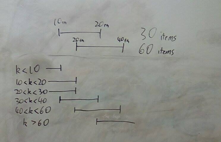
This is a diagram of what happens when one data structure has 30 items and the other has 60 items. It contains all of the different cases for $k$. For example, when $k$ is 35, then we can discard the upper and lower thirds of the 30 item data structure, and we can discard the upper third of the 60 item data structure.

You can draw similar diagrams for the other cases.

This part is the sketchiest part of the whole algorithm. I’m pretty sure that you can always decrease at least one of the data structures by one third. I’m not sure if you can always shrink both of them. I’m not sure how much you can shrink the OST in constant time; I’m pretty sure you can do at least $\frac 16$, and I think that for any fraction less than $\frac 13$, you can choose a node depth such that you can always cut that fraction out in constant time.

Runtime of this solution

If one of the data structures starts out much larger than the other one, it will shrink until they’re similar sizes. This takes $O(m)$ time for the array and $O(\log(n))$ time for the OST.

Once they’re the same size, I think that at least one of them will both shrink by one third every time. So we have the recurrence relation:

$^$f(n, m) = f \left( \frac {2n}3, \frac {2m}3\right) + m + 1$^$

which evaluates to $\log(n) + m$.

Conclusion

So we can do quick select on an OST and array at the same time in $O(m + \log(n))$.

My work here leaves a lot to be desired. Most obviously, my fastest algorithm is extremely complicated and inelegant; I bet that can be simplified.